pandas, matplotlib, seaborn 모듈 활용하기
06 Jan 2018 | 머신러닝 Python여기서 사용한 테스트 데이터는 여기에서 받을 수 있습니다.
Pandas
pandas는 많은 데이터를 쉽게 다룰 수 있는 기능을 제공하는 Python 모듈입니다.
예제 코드
import pandas as pd

data_set = pd.read_csv('pima-indians-diabetes.csv',
                       names=["pregnant", "plasma", "presure", "thickness",
                              "insulin", "BMI", "pedigree", "age", "class"])

print(data_set.head(5))

print('====================================================================\n')

print(data_set.info())

print('====================================================================\n')

print(data_set.describe())
data_set.head(5)는 상위 5개의 데이터들의 리스트를 조회하는 명령어입니다. 또한 info() 함수를 이용해서 각 정보들의 데이터 타입이나 데이터 개수 등을 확인할 수 있고, describe() 함수를 이용해서 정보별 샘플의 개수, 평균, 표준 편차, 최소/최대값 등을 조회할 수 있습니다.
실행 결과
   pregnant  plasma  presure  thickness  insulin   BMI  pedigree  age  class
0         6     148       72         35        0  33.6     0.627   50      1
1         1      85       66         29        0  26.6     0.351   31      0
2         8     183       64          0        0  23.3     0.672   32      1
3         1      89       66         23       94  28.1     0.167   21      0
4         0     137       40         35      168  43.1     2.288   33      1
==================================================================================

<class 'pandas.core.frame.DataFrame'>
RangeIndex: 768 entries, 0 to 767
Data columns (total 9 columns):
pregnant     768 non-null int64
plasma       768 non-null int64
presure      768 non-null int64
thickness    768 non-null int64
insulin      768 non-null int64
BMI          768 non-null float64
pedigree     768 non-null float64
age          768 non-null int64
class        768 non-null int64
dtypes: float64(2), int64(7)
memory usage: 54.1 KB
None
==================================================================================

         pregnant      plasma     presure   thickness     insulin         BMI  \
count  768.000000  768.000000  768.000000  768.000000  768.000000  768.000000
mean     3.845052  120.894531   69.105469   20.536458   79.799479   31.992578
std      3.369578   31.972618   19.355807   15.952218  115.244002    7.884160
min      0.000000    0.000000    0.000000    0.000000    0.000000    0.000000
25%      1.000000   99.000000   62.000000    0.000000    0.000000   27.300000
50%      3.000000  117.000000   72.000000   23.000000   30.500000   32.000000
75%      6.000000  140.250000   80.000000   32.000000  127.250000   36.600000
max     17.000000  199.000000  122.000000   99.000000  846.000000   67.100000

         pedigree         age       class
count  768.000000  768.000000  768.000000
mean     0.471876   33.240885    0.348958
std      0.331329   11.760232    0.476951
min      0.078000   21.000000    0.000000
25%      0.243750   24.000000    0.000000
50%      0.372500   29.000000    0.000000
75%      0.626250   41.000000    1.000000
max      2.420000   81.000000    1.000000
matplotlib, seaborn
matplotlib은 Python에서 그래프를 그리기 쉽도록 해주는 모듈입니다. 그리고 seaborn 모듈은 각 정보들끼리의 상관관계를 쉽게 볼 수 있도록 해줍니다.
Heatmap 예제 코드
import pandas as pd
import matplotlib.pyplot as plt
import seaborn as sns

data_set = pd.read_csv('pima-indians-diabetes.csv',
                       names=["pregnant", "plasma", "presure", "thickness",
                              "insulin", "BMI", "pedigree", "age", "class"])

# 그래프의 크기 지정
plt.figure(figsize=(8, 8))

# Heatmap 설정
sns.heatmap(data_set.corr(), linewidths=0.1, vmax=0.5, cmap=plt.cm.gist_heat,
            linecolor='white', annot=True)

# 렌더링
plt.show()
실행 결과
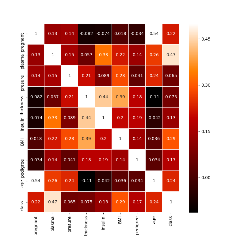
Heatmap을 이용하면 각 속성들간의 상관관계 크기를 알 수 있습니다. 위 결과에서는 plasma 항목과 class의 항목의 상관관계가 높은 것을 확인할 수 있습니다.
Grid 예제 코드
import pandas as pd
import matplotlib.pyplot as plt
import seaborn as sns

data_set = pd.read_csv('pima-indians-diabetes.csv',
                       names=["pregnant", "plasma", "presure", "thickness",
                              "insulin", "BMI", "pedigree", "age", "class"])

grid = sns.FacetGrid(data_set, col='class')
grid.map(plt.hist, 'plasma', bins=10)

plt.show()
실행 결과
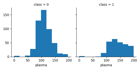
위 그래프를 보면 class 속성이 1인 경우(위 데이터는 당뇨병 환자를 의미하는 속성) plasma 항목의 수치가 150 이상일 때, class = 0일 때의 경우와 다르다는 것을 확인할 수 있습니다.